如何训练属于自己的目标检测模型

YOLO，You Only Look Once，是目前应用最广泛的基于深度学习的目标检测算法之一。在当前大模型逐渐成为主流时，在目标检测领域依然非常能打。目前Yolo已经被ultralytics更新到了V8，有了更先进的跟踪检测算法。但在先前项目有目标检测需求时，Yolov5还是主流，彼时也仅仅由美团更新到了v6。因此以下文章所用的版本均为Yolov5。

准备代码环境

相对于Yolov8可以之间pip安装的便捷，Yolov5则需要克隆对于的代码库并安装其依赖性。推荐使用Sudo权限来安装依赖包。

git clone https://github.com/ultralytics/yolov5

我建议使用新的conda或者virtualenv environment,前者安装Anaconda3即可，后者如果你使用pycharm这一类型的ide也会自带一个虚拟环境的管理器。使用这一类型的环境虚拟化管理器可以有效的避免搞乱现有的项目依赖环境。本文这使用的Conda来运行本项目依赖。

conda create -n yolov5 python=3.7
conda activate yolov5
cd yolov5
pip install -r requirements.txt

准备好源码仓库以及依赖后让我们来继续准备所需训练的数据集吧

准备数据集

介于本文只是简单的演示，于是数据集选取了网上公开的小数据集，将使用来自 MakeML 的道路标志目标检测数据集。包含了一些道路标志，整体数据量相对于工作中实际数据量要小很多很多。仅仅包含了4类道路提示以及877个小图像。我们可以从Kaggle获取该数据集。

下载数据集

在yolov5同目录下创建Road_Sign_Dataset文件夹，用来存放数据集

1. 登录Kaggle，在Settings中Create New Token 即可获得一个包含token的json文件。
2. 运行pip install kaggle命令安装kaggle依赖，并将包含Token的json文件放置在用户目录下的.kaggle文件夹下
3. 在Road_Sign_Dataset文件夹内下载对应数据集 kaggle datasets download andrewmvd/road-sign-detection
4. 解压文件 unzip road-sign-detection.zip
5. 删除源文件 rm -r road-sign-detection.zip

使用labelimg查看数据集

得到数据集文件后我们可以使用一些标签标注工具比如Labelme,labelimg以及前段时间比较火的结合SAM模型分割的一些标注工具如 Label-Studio来打开数据集，可以直观的查看数据集的标注的内容。我们仅仅查看数据集，这里简单的安装一下labelimg即可.

conda create --name=labelimg python=3.9
conda activate labelimg
pip install PyQt5 pyqt5-tools lxml labelimg
labelimg

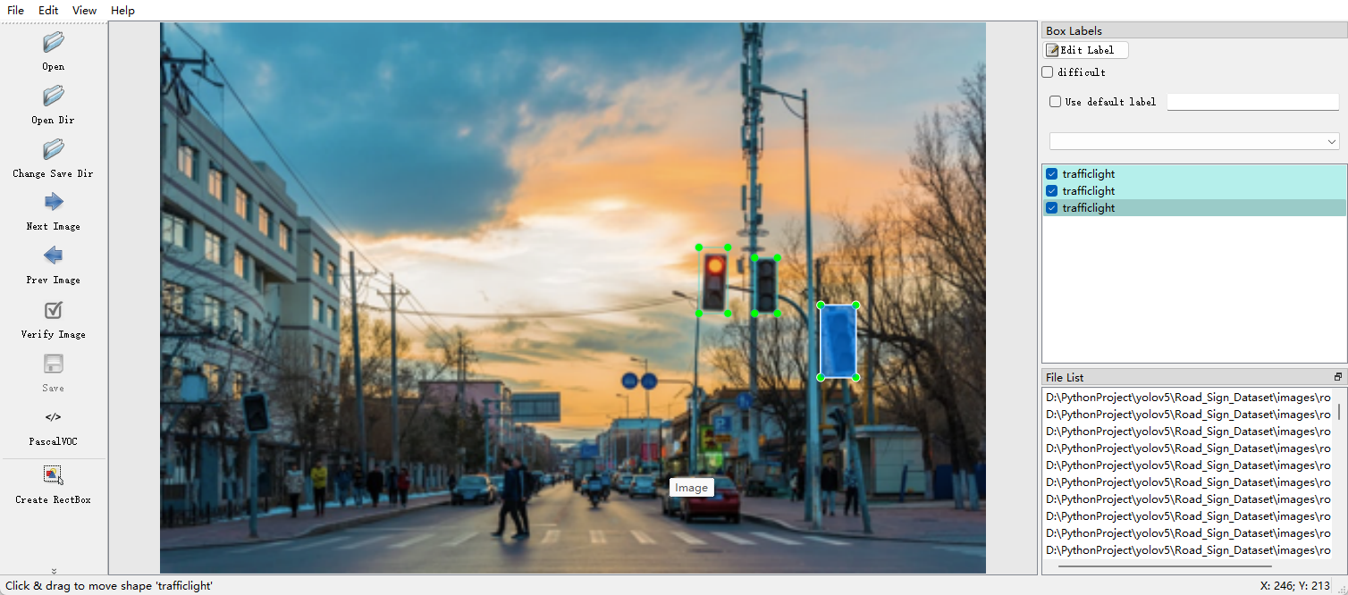
打开labelimg后选择对应的数据集文件夹以及标注数据的文件夹即可直观的看见标注效果

注释格式转换

现在我们以及拥有一个VOC格式(这是一种非常常见的存储在XML中文件中的注释格式)的路标数据集，但是VOC格式的数据集是无法直接提供给YOLOv5训练解析的，我们需要编写脚本将其转化为Yolo注释的格式。

首先我们先来看看上图对应的标注文件road25.xml内VOC格式的注释格式。

<annotation>
    <folder>images</folder>
    <filename>road25.png</filename>
    <size>
        <width>400</width>
        <height>267</height>
        <depth>3</depth>
    </size>
    <segmented>0</segmented>
    <object>
        <name>trafficlight</name>
        <pose>Unspecified</pose>
        <truncated>0</truncated>
        <occluded>0</occluded>
        <difficult>0</difficult>
        <bndbox>
            <xmin>261</xmin>
            <ymin>109</ymin>
            <xmax>275</xmax>
            <ymax>141</ymax>
        </bndbox>
    </object>
    <object>
        <name>trafficlight</name>
        <pose>Unspecified</pose>
        <truncated>0</truncated>
        <occluded>0</occluded>
        <difficult>0</difficult>
        <bndbox>
            <xmin>288</xmin>
            <ymin>114</ymin>
            <xmax>299</xmax>
            <ymax>141</ymax>
        </bndbox>
    </object>
    <object>
        <name>trafficlight</name>
        <pose>Unspecified</pose>
        <truncated>0</truncated>
        <occluded>0</occluded>
        <difficult>0</difficult>
        <bndbox>
            <xmin>320</xmin>
            <ymin>137</ymin>
            <xmax>337</xmax>
            <ymax>172</ymax>
        </bndbox>
    </object>
</annotation>

这个注释文件描述了图片的文件夹名称，文件名，图片分辨率大小。以及注释了包含的对象，以及通过坐标框选了对象的位置。而Yolo格式的注释首先是存储在TxT中。每一行都包含了一个VOC中的一个框选的对象。先贴一张来自官网的图来解释一下yolo的注释格式

注释文件具体内容如下

0 0.670 0.468 0.035 0.120
0 0.734 0.478 0.028 0.101
0 0.821 0.579 0.043 0.131

一共标注了三个对象（三个红绿灯）。每一行代表这些对象中的一个。规范如下。

• 每个对象一行
• 每一行 格式为 对象类别 x中心 y中心 宽的比值 高的比值（坐标必须按照图像的尺寸进行标准化）
• 对象类别是类索引下标(从0开始)。

将VOC格式数据转化为Yolo格式数据需要提取的有用信息为 标注对象类别，标注对象的坐标。我们写一个函数来从Voc注释文件中批量提取这两个信息。

import xml.etree.ElementTree as ET

# 该函数从XML注释中获取标注数据
def extract_info_from_xml(xml_file):
    root = ET.parse(xml_file).getroot()
    
    # 初始化标注信息字典
    info_dict = {}
    info_dict['bboxes'] = []

    # 解析XML树
    for elem in root:
        # 获取图片名称
        if elem.tag == "filename":
            info_dict['filename'] = elem.text
            
        # 获取图片大小尺寸
        elif elem.tag == "size":
            image_size = []
            for subelem in elem:
                image_size.append(int(subelem.text))
            
            info_dict['image_size'] = tuple(image_size)
        
        # 获取标注边界框的详细信息
        elif elem.tag == "object":
            bbox = {}
            for subelem in elem:
                if subelem.tag == "name":
                    bbox["class"] = subelem.text
                elif subelem.tag == "bndbox":
                    for subsubelem in subelem:
                        bbox[subsubelem.tag] = int(subsubelem.text)            
            info_dict['bboxes'].append(bbox)
    
    return info_dict

该函数返回一个包含了VOC中标注的所有对象的 类别与坐标的字典。

接下来我们需要根据字典的生成Yolo格式的注释文件，现在我们编写convert_to_yolov5(info_dict)函数，转换格式并写入TXT中。

# 将标注对象分别映射到id的字典（可动态获取）
class_name_to_id_mapping = {"trafficlight": 0,
                           "stop": 1,
                           "speedlimit": 2,
                           "crosswalk": 3}

# 将上一步的包含标注对象信息字典转换为yolo的格式并将其写入txt
def convert_to_yolov5(info_dict):
    print_buffer = []
    
    # 遍历每一个对象标注框
    for b in info_dict["bboxes"]:
        try:
            class_id = class_name_to_id_mapping[b["class"]]
        except KeyError:
            print("无效的类型", class_name_to_id_mapping.keys())
        
        # 将Voc格式的坐标转换为Yolo的格式（Yolo的标注为矩形框，转化为矩形中心点坐标以及长宽相对于整个图片的比即可）
        b_center_x = (b["xmin"] + b["xmax"]) / 2 
        b_center_y = (b["ymin"] + b["ymax"]) / 2
        b_width    = (b["xmax"] - b["xmin"])
        b_height   = (b["ymax"] - b["ymin"])
        
        # 转化为统一的比值表示
        image_w, image_h, image_c = info_dict["image_size"]  
        b_center_x /= image_w 
        b_center_y /= image_h 
        b_width    /= image_w 
        b_height   /= image_h 
        
        #按yolo格式添加进数组
        print_buffer.append("{} {:.3f} {:.3f} {:.3f} {:.3f}".format(class_id, b_center_x, b_center_y, b_width, b_height))
        
    #拼接文件名
    save_file_name = os.path.join("annotations", info_dict["filename"].replace("png", "txt"))
    
    # 持久化到磁盘
    print("\n".join(print_buffer), file= open(save_file_name, "w"))

现在我们将所有 VOL转换为 YOLO 样式的 txt 注释。

# 获取vol注释的文件
annotations = [os.path.join('annotations', x) for x in os.listdir('annotations') if x[-3:] == "xml"]
annotations.sort()

# 调用先前的函数转化并保存
for ann in tqdm(annotations):
    info_dict = extract_info_from_xml(ann)
    convert_to_yolov5(info_dict)
annotations = [os.path.join('annotations', x) for x in os.listdir('annotations') if x[-3:] == "txt"]

划分数据集

将VOC格式转化为Yolo格式化后，这个数据集并不能直接用来训练，我们还需要将这个数据集划分为三份。分别是训练集，验证集，与测试集，常见的会将大量的样本放在训练集，少量放在验证集或者测试集，甚至测试集合不放，所以常见比例为 7:2:1或者 8:1:1,甚至为 8:2:0接下来我们编写脚本分别数据集根据8:1:1的比例划分好数据集。划分好数据集后数据集准备工作基本完成了。这里就贴出完整代码好了。

import torch
from IPython.display import Image  # for displaying images
import os 
import random
import shutil
from sklearn.model_selection import train_test_split
import xml.etree.ElementTree as ET
from xml.dom import minidom
from tqdm import tqdm
from PIL import Image, ImageDraw
import numpy as np
import matplotlib.pyplot as plt

# 将标注对象分别映射到id的字典（可动态获取）
class_name_to_id_mapping = {"trafficlight": 0,
                           "stop": 1,
                           "speedlimit": 2,
                           "crosswalk": 3}
random.seed(108)

# 该函数从XML注释中获取标注数据
def extract_info_from_xml(xml_file):
    root = ET.parse(xml_file).getroot()
    # 初始化标注信息字典
    info_dict = {}
    info_dict['bboxes'] = []
    # 解析XML树
    for elem in root:
        # 获取图片名称
        if elem.tag == "filename":
            info_dict['filename'] = elem.text
        # 获取图片大小尺寸
        elif elem.tag == "size":
            image_size = []
            for subelem in elem:
                image_size.append(int(subelem.text))
            info_dict['image_size'] = tuple(image_size)
        # Get details of the bounding box 
        elif elem.tag == "object":
            bbox = {}
            for subelem in elem:
                if subelem.tag == "name":
                    bbox["class"] = subelem.text
                elif subelem.tag == "bndbox":
                    for subsubelem in subelem:
                        bbox[subsubelem.tag] = int(subsubelem.text)            
            info_dict['bboxes'].append(bbox)
    return info_dict

# 将上一步的包含标注对象信息字典转换为yolo的格式并将其写入txt
def convert_to_yolov5(info_dict):
    print_buffer = []
    # 遍历每一个对象标注框
    for b in info_dict["bboxes"]:
        try:
            class_id = class_name_to_id_mapping[b["class"]]
        except KeyError:
            print("无效的类型", class_name_to_id_mapping.keys())
        # 将Voc格式的坐标转换为Yolo的格式（Yolo的标注为矩形框，转化为矩形中心点坐标以及长宽相对于整个图片的比即可）
        b_center_x = (b["xmin"] + b["xmax"]) / 2 
        b_center_y = (b["ymin"] + b["ymax"]) / 2
        b_width    = (b["xmax"] - b["xmin"])
        b_height   = (b["ymax"] - b["ymin"])
        # 转化为统一的比值表示
        image_w, image_h, image_c = info_dict["image_size"]  
        b_center_x /= image_w 
        b_center_y /= image_h 
        b_width    /= image_w 
        b_height   /= image_h 
        #按yolo格式添加进数组
        print_buffer.append("{} {:.3f} {:.3f} {:.3f} {:.3f}".format(class_id, b_center_x, b_center_y, b_width, b_height))
        
    #拼接文件名
    save_file_name = os.path.join("annotations", info_dict["filename"].replace("png", "txt"))
    # 持久化到磁盘
    print("\n".join(print_buffer), file= open(save_file_name, "w"))
    #删除源文件
    os.remove(os.path.join("annotations", info_dict["filename"].replace("png", "xml")))
# 创建目录
def create_yolo_folder():
    os.mkdir(".\\images\\train")
    os.mkdir(".\\images\\val")
    os.mkdir(".\\images\\test")
    os.mkdir(".\\annotations\\train")
    os.mkdir(".\\annotations\\val")
    os.mkdir(".\\annotations\\test")
#移动图片
def move_files_to_folder(list_of_files, destination_folder):
    for f in list_of_files:
        try:
            shutil.move(f, destination_folder)
        except:
            print(f)
            assert False 
#函数入口
if __name__ =='__main__': 
    # 获取vol注释的文件
    annotations = [os.path.join('annotations', x) for x in os.listdir('annotations') if x[-3:] == "xml"]
    annotations.sort()
    # 调用先前的函数转化并保存
    for ann in tqdm(annotations):
        info_dict = extract_info_from_xml(ann)
        convert_to_yolov5(info_dict)
    annotations = [os.path.join('annotations', x) for x in os.listdir('annotations') if x[-3:] == "txt"]
    # 读取图片与标注注释文件
    images = [os.path.join('images', x) for x in os.listdir('images')]
    annotations = [os.path.join('annotations', x) for x in os.listdir('annotations') if x[-3:] == "txt"]
    images.sort()
    annotations.sort()
    # 根据 训练集，验证集，与测试集 划分数据集
    train_images, val_images, train_annotations, val_annotations = train_test_split(images, annotations, test_size = 0.2, random_state = 1)
    val_images, test_images, val_annotations, test_annotations = train_test_split(val_images, val_annotations, test_size = 0.5, random_state = 1)
    create_yolo_folder()
    # 移动切分好的数据集
    move_files_to_folder(train_images, 'images/train')
    move_files_to_folder(val_images, 'images/val/')
    move_files_to_folder(test_images, 'images/test/')
    move_files_to_folder(train_annotations, 'annotations/train/')
    move_files_to_folder(val_annotations, 'annotations/val/')
    move_files_to_folder(test_annotations, 'annotations/test/')
    # 修改文件夹名称为yolo注释的文件夹名
    os.rename('annotations','labels')

训练

准备好数据集后接下来就是我们的重头戏，训练数据集了。数据集的训练我们可以从官方选择一个预训练模型进行训练。本文仅仅为了演示，故而选择的是对性能要求最小的n模型。

以下是各个版本官方给出的参数表格

Model	size (pixels)	mAPval 0.5:0.95	mAPval 0.5	Speed CPU b1 (ms)	Speed V100 b1 (ms)	Speed V100 b32 (ms)	params (M)	FLOPs @640 (B)
YOLOv5n	640	28.0	45.7	45	6.3	0.6	1.9	4.5
YOLOv5s	640	37.4	56.8	98	6.4	0.9	7.2	16.5
YOLOv5m	640	45.4	64.1	224	8.2	1.7	21.2	49.0
YOLOv5l	640	49.0	67.3	430	10.1	2.7	46.5	109.1
YOLOv5x	640	50.7	68.9	766	12.1	4.8	86.7	205.7
YOLOv5n6	1280	36.0	54.4	153	8.1	2.1	3.2	4.6
YOLOv5s6	1280	44.8	63.7	385	8.2	3.6	12.6	16.8
YOLOv5m6	1280	51.3	69.3	887	11.1	6.8	35.7	50.0
YOLOv5l6	1280	53.7	71.3	1784	15.8	10.5	76.8	111.4
YOLOv5x6 + TTA	1280 1536	55.0 55.8	72.7 72.7	3136 -	26.2 -	19.4 -	140.7 -	209.8 -

我们使用train.py 来训练数据集，而train关于训练有如下常用参数

• batch: 批量处理的数目,根据训练显卡的显存来调节，最好训练时可以吃比较多的显存又不至于爆显存

• epochs: 需要训练的轮次，常用轮次为300轮 （次数太少效果会很差，次数太多会过拟合）

• data: 数据 YAML 文件，包含有关数据集的信息(图像路径、标签)

• cfg: 模型架构。有5种选择: yolo5n.yaml,yolo5s.yaml，yolov5m.yaml，yolov5l.yaml，yolov5x.yaml。这些模型的大小和复杂程度按升序增加，你可以选择一个适合你目标检测任务复杂程度的模型。如果希望使用自定义体系结构，则必须在指定网络体系结构的 model 文件夹中定义 YAML 文件。本文使用的n模型仅仅为了演示效果，实际上n模型只有在移动端上这种硬件性能极差的情况下才会考虑n模型，其他场景几乎没有遇见过使用情况，业务中常用的为Medium与Large模型。

• weights: 使用预训练模型，没有预训练模型可以使用官方的即可

• hyp: hyperparameter,超参数文件 一般不用修改

• name: 关于训练的各种事情，如训练日志。训练重量将存储在名为 run/train/name 的文件夹中

接下来详细的说明一些配置文件。

数据集信息

​ data参数将会指向一个数据集相关配置信息的Yaml文件，必须在数据集配置文件中定义以下参数:

1. train, test, and val:训练集，测试集与验证集的图片文件夹的位置

2. nc: 数据集中的对象的数目。

3. names: 数据集中的类的名称。此列表中的类的索引下标将用作代码中类名的标识符。因此列表的中各个类型的顺序必须与标注文件中的类索引下标一致

   根据本文中的road_sign_data数据集创建一个名为 road_sign_data. yaml 的配置文件，并将其放在 yolov5/data 文件夹中。内容如下

   train: ../Road_Sign_Dataset/images/train/ 
   val:  ../Road_Sign_Dataset/images/val/
   test: ../Road_Sign_Dataset/images/test/
   # number of classes
   nc: 4
   # class names
   names: ["trafficlight","stop", "speedlimit","crosswalk"]

模型网络架构

Yolov5还允许您定义自己的定制架构和锚，如果预定的网络架构不适合，也可以自定义权重配置文件。本文中我们使用 yolov5n.yaml。内容如下，简单修改一下nc值为类型数量即可。训练时使用cfg指定即可

# YOLOv5 🚀 by Ultralytics, AGPL-3.0 license

# Parameters
nc: 4  # number of classes
depth_multiple: 0.33  # model depth multiple
width_multiple: 0.25  # layer channel multiple
anchors:
  - [10,13, 16,30, 33,23]  # P3/8
  - [30,61, 62,45, 59,119]  # P4/16
  - [116,90, 156,198, 373,326]  # P5/32

# YOLOv5 v6.0 backbone
backbone:
  # [from, number, module, args]
  [[-1, 1, Conv, [64, 6, 2, 2]],  # 0-P1/2
   [-1, 1, Conv, [128, 3, 2]],  # 1-P2/4
   [-1, 3, C3, [128]],
   [-1, 1, Conv, [256, 3, 2]],  # 3-P3/8
   [-1, 6, C3, [256]],
   [-1, 1, Conv, [512, 3, 2]],  # 5-P4/16
   [-1, 9, C3, [512]],
   [-1, 1, Conv, [1024, 3, 2]],  # 7-P5/32
   [-1, 3, C3, [1024]],
   [-1, 1, SPPF, [1024, 5]],  # 9
  ]

# YOLOv5 v6.0 head
head:
  [[-1, 1, Conv, [512, 1, 1]],
   [-1, 1, nn.Upsample, [None, 2, 'nearest']],
   [[-1, 6], 1, Concat, [1]],  # cat backbone P4
   [-1, 3, C3, [512, False]],  # 13

   [-1, 1, Conv, [256, 1, 1]],
   [-1, 1, nn.Upsample, [None, 2, 'nearest']],
   [[-1, 4], 1, Concat, [1]],  # cat backbone P3
   [-1, 3, C3, [256, False]],  # 17 (P3/8-small)

   [-1, 1, Conv, [256, 3, 2]],
   [[-1, 14], 1, Concat, [1]],  # cat head P4
   [-1, 3, C3, [512, False]],  # 20 (P4/16-medium)

   [-1, 1, Conv, [512, 3, 2]],
   [[-1, 10], 1, Concat, [1]],  # cat head P5
   [-1, 3, C3, [1024, False]],  # 23 (P5/32-large)

   [[17, 20, 23], 1, Detect, [nc, anchors]],  # Detect(P3, P4, P5)
  ]

超参数

超参数配置文件内容为神经网络定义超参数。一般情况下使用默认值即可，默认的配置文件在data/hyps。

# YOLOv5 🚀 by Ultralytics, AGPL-3.0 license
# Hyperparameters for low-augmentation COCO training from scratch
# python train.py --batch 64 --cfg yolov5n6.yaml --weights '' --data coco.yaml --img 640 --epochs 300 --linear
# See tutorials for hyperparameter evolution https://github.com/ultralytics/yolov5#tutorials

lr0: 0.01  # initial learning rate (SGD=1E-2, Adam=1E-3)
lrf: 0.01  # final OneCycleLR learning rate (lr0 * lrf)
momentum: 0.937  # SGD momentum/Adam beta1
weight_decay: 0.0005  # optimizer weight decay 5e-4
warmup_epochs: 3.0  # warmup epochs (fractions ok)
warmup_momentum: 0.8  # warmup initial momentum
warmup_bias_lr: 0.1  # warmup initial bias lr
box: 0.05  # box loss gain
cls: 0.5  # cls loss gain
cls_pw: 1.0  # cls BCELoss positive_weight
obj: 1.0  # obj loss gain (scale with pixels)
obj_pw: 1.0  # obj BCELoss positive_weight
iou_t: 0.20  # IoU training threshold
anchor_t: 4.0  # anchor-multiple threshold
# anchors: 3  # anchors per output layer (0 to ignore)
fl_gamma: 0.0  # focal loss gamma (efficientDet default gamma=1.5)
hsv_h: 0.015  # image HSV-Hue augmentation (fraction)
hsv_s: 0.7  # image HSV-Saturation augmentation (fraction)
hsv_v: 0.4  # image HSV-Value augmentation (fraction)
degrees: 0.0  # image rotation (+/- deg)
translate: 0.1  # image translation (+/- fraction)
scale: 0.5  # image scale (+/- gain)
shear: 0.0  # image shear (+/- deg)
perspective: 0.0  # image perspective (+/- fraction), range 0-0.001
flipud: 0.0  # image flip up-down (probability)
fliplr: 0.5  # image flip left-right (probability)
mosaic: 1.0  # image mosaic (probability)
mixup: 0.0  # image mixup (probability)
copy_paste: 0.0  # segment copy-paste (probability)

训练模型

在上述的配置文件中定义了 数据集位置，类的数量与名称后，即可直接使用命令开始训练了。由于设备受限，无论是数据集的选择是少量的小图片，模型的选择也选择了n模型。这次训练批量处理的数目为32，训练轮次为100.

单卡

python train.py --img 640 --cfg models/yolov5n.yaml --hyp hyp.scratch.yaml --batch 32 --epochs 100 --data data/road_sign_data.yaml --weights yolov5n.pt --workers 24 --name yolo_road_det

多卡训练

python  train.py  --img 640 --cfg models/yolov5n.yaml --hyp hyp.scratch.yaml --batch 32 --epochs 100 --data data/road_sign_data.yaml --weights yolov5n.pt --workers 24 --name yolo_road_det  --device 0,1

缺点：这种方法很慢，与仅使用 1 个 GPU 相比，几乎无法加快训练速度。大部分压力依旧在GPU1上,因此仅推荐在Windows中使用

推荐：

python -m torch.distributed.run --nproc_per_node 2  train.py  --img 640 --cfg models/yolov5n.yaml --hyp hyp.scratch.yaml --batch 32 --epochs 100 --data data/road_sign_data.yaml --weights yolov5n.pt --workers 24 --name yolo_road_det --device 0,1

在训练时可以使用nvidia-smi查看实时的显存使用情况，再适当调节batch的值，充分榨干显卡。

训练完毕后，训练好的数据会保存在.\runs\train\yolo_road_det2中，模型在weights文件夹下的best.pt

推理

python detect.py --source 0  # webcam
                            file.jpg  # image 
                            file.mp4  # video
                            path/  # directory
                            path/*.jpg  # glob
                            rtsp://170.93.143.139/rtplive/470011e600ef003a004ee33696235daa  # rtsp stream
                            rtmp://192.168.1.105/live/test  # rtmp stream
                            http://112.50.243.8/PLTV/88888888/224/3221225900/1.m3u8  # http stream